Chapter 12 Lab 11: Computational Data Fitting and Predictive Modeling
Objectives:
- To fit a linear regression model in R
- To interpret model coefficients, R-squared, and p-values
- To evaluate model fit using residuals
- To use a fitted model to forecast/predict new values
This is our final statistics lab of the semester. Instead of just testing whether groups differ (Labs 6 and 10), today we build a model that describes how one variable changes as another changes — and use it to make predictions, a common task in environmental and conservation biology (e.g., forecasting population trends or growth curves).
12.1 Linear regression basics
A simple linear regression models a straight-line relationship:
\[y = \beta_0 + \beta_1 x + \epsilon\]
where \(\beta_0\) is the intercept, \(\beta_1\) is the slope, and \(\epsilon\) is the error term.
Let’s use body measurements from the penguins data set (Lab 4/9) to model how flipper length predicts body mass.
##
## Call:
## lm(formula = body_mass_g ~ flipper_length_mm, data = penguins)
##
## Residuals:
##      Min       1Q   Median       3Q      Max
## -1057.33  -259.79   -12.24   242.97  1293.89
##
## Coefficients:
##                   Estimate Std. Error t value Pr(>|t|)
## (Intercept)       -5872.09     310.29  -18.93   <2e-16 ***
## flipper_length_mm    50.15       1.54   32.56   <2e-16 ***
## ---
## Signif. codes:  0 '***' 0.001 '**' 0.01 '*' 0.05 '.' 0.1 ' ' 1
##
## Residual standard error: 393.3 on 331 degrees of freedom
## Multiple R-squared:  0.7621, Adjusted R-squared:  0.7614
## F-statistic:  1060 on 1 and 331 DF,  p-value: < 2.2e-16
Key parts of the output:
- Estimate (Intercept and slope): the fitted values of \(\beta_0\) and \(\beta_1\)
- Pr(>|t|): p-value testing whether each coefficient differs significantly from zero
- R-squared: the proportion of variance in \(y\) explained by \(x\) (0 to 1; closer to 1 = better fit)
Question 1
- What is the slope of this model? In plain language, what does it mean biologically (e.g., “for every 1mm increase in flipper length, body mass increases by ___ grams”)?
- What is the R-squared value? How much of the variation in body mass does flipper length explain?
- Is the slope statistically significant? How do you know?
12.2 Visualizing the fitted line
ggplot(data = penguins, aes(x = flipper_length_mm, y = body_mass_g)) +
  geom_point() +
  geom_smooth(method = "lm", se = TRUE) +
  labs(x = "Flipper length (mm)", y = "Body mass (g)") +
  theme_minimal()
## `geom_smooth()` using formula = 'y ~ x'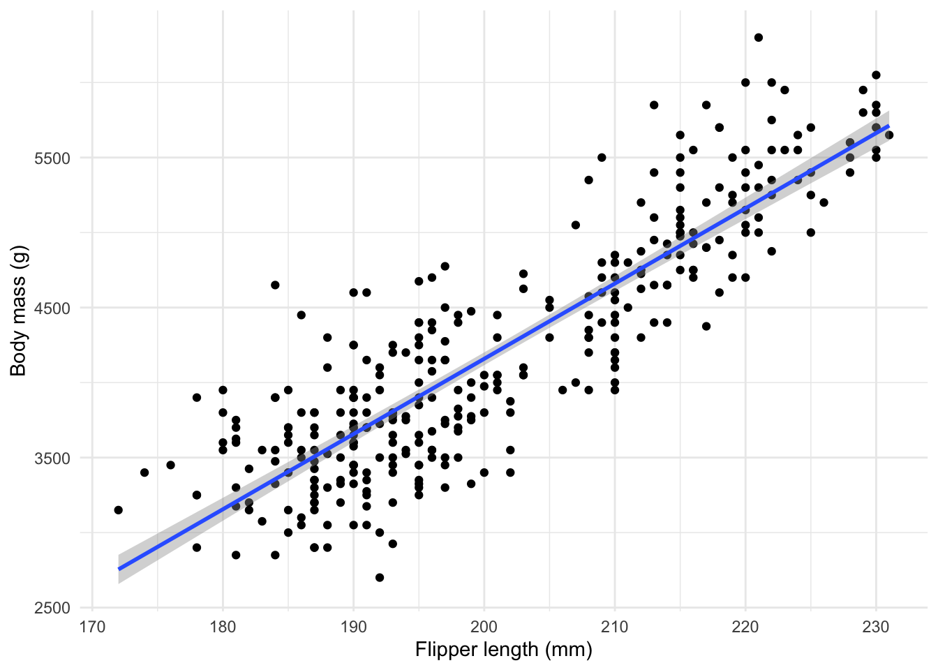
geom_smooth(method="lm") overlays the regression line, and se=TRUE shades a 95% confidence band around it.
Question 2
-
Recreate this plot but colored by
species. Does the flipper length - body mass relationship look consistent across species, or different?
12.3 Checking the fit: residuals
Residuals are the differences between observed and predicted values (\(y_{observed} - y_{predicted}\)). A good linear fit should have residuals scattered randomly around zero, with no obvious pattern.
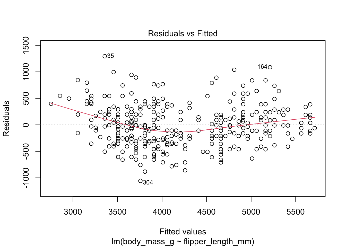
If you see a clear curve or funnel shape in this plot, a straight line may not be the right model for your data.
Question 3
- Based on the residual plot, does a linear model seem like a reasonable fit for this relationship? Explain what you’d look for to answer “yes” or “no.”
12.4 Making predictions
Once a model is fit, you can use it to predict new, unobserved values with predict():
##        1
## 4660.093
Question 4
- Using your fitted model, predict the body mass of a penguin with a flipper length of 195mm and one with 225mm
-
One of these predictions is likely more reliable than the other.
Which one, and why? (Hint: look at the range of flipper lengths actually
observed in the data with
range(penguins$flipper_length_mm)— predicting outside this range is called “extrapolation”)
12.5 Curve fitting for growth and conservation trends
Not all biological relationships are straight lines. Population growth, for example, is often better modeled with a curve. Here’s a simple example using nls() (nonlinear least squares) to fit an exponential growth curve to simulated population data:
set.seed(11)
year <- 1:15
population <- 50 * exp(0.15 * year) + rnorm(15, 0, 10)
pop_data <- data.frame(year, population)

growth_model <- nls(population ~ N0 * exp(r * year), data = pop_data,
                     start = list(N0 = 50, r = 0.1))
summary(growth_model)
##
## Formula: population ~ N0 * exp(r * year)
##
## Parameters:
## Estimate Std. Error t value Pr(>|t|)
## N0 49.23624 2.16641 22.73 7.53e-12 ***
## r 0.14961 0.00348 42.99 2.11e-15 ***
## ---
## Signif. codes: 0 '***' 0.001 '**' 0.01 '*' 0.05 '.' 0.1 ' ' 1
##
## Residual standard error: 9.213 on 13 degrees of freedom
##
## Number of iterations to convergence: 4
## Achieved convergence tolerance: 3.79e-06ggplot(pop_data, aes(x = year, y = population)) +
geom_point() +
geom_line(aes(y = predict(growth_model)), color = "blue") +
labs(title = "Fitted exponential growth curve", x = "Year", y = "Population size") +
theme_minimal()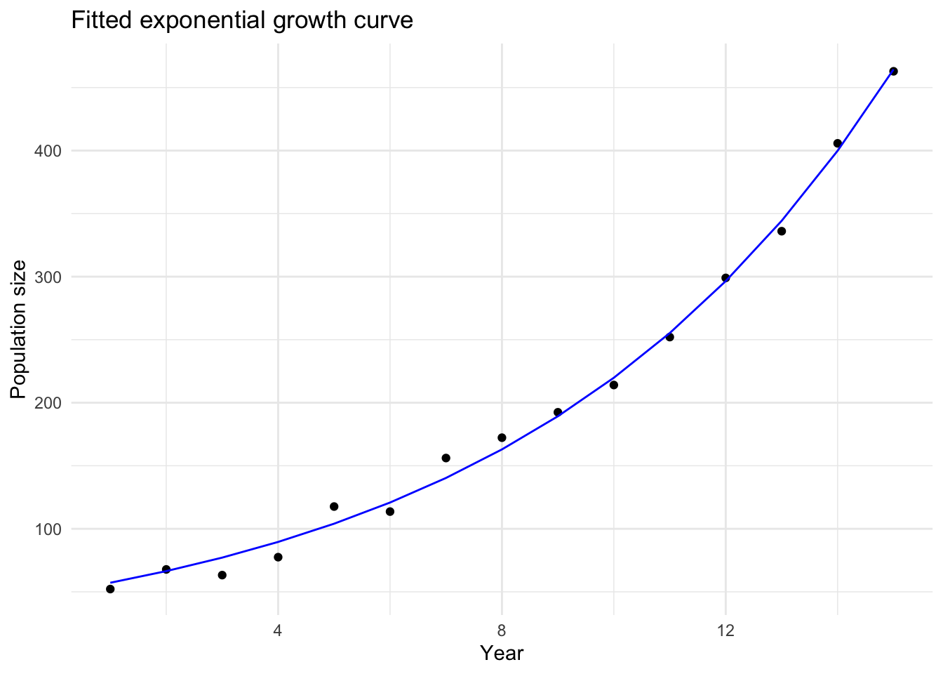
Question 5
-
What is the fitted growth rate (\(r\)) from
growth_model? -
Use
predict()with this model to forecast the population size at year 20. Add the code and result. - Why might a linear model be a poor choice for forecasting population growth, compared to this exponential model? Relate your answer back to what you observed with residuals in Question 3.